
Supervised and Unsupervised Machine Learning Primer Understanding Supervised Learning Examples of Supervised Learning Algorithms Examples of Unsupervised Learning In Summary: About Chisel Analytics:
Supervised and unsupervised learning algorithms are often the first two ‘families’ of techniques introduced in machine learning classrooms and textbooks. So, what are they?
Understanding Supervised Learning
Supervised learning algorithms attempt to predict some label or value for a given observation. This could take many forms — from predicting the value of a home to classifying a music track by genre.
The key to supervised learning algorithms is that they require previous examples where you know the label or value you wish to predict.
For predicting home value, you would need a spreadsheet of real estate sales data and details about them, including number of bedrooms, bathrooms, amenities, square footage, and location. For classifying music genres, you would need details for a library of songs including tempo, pitch, and timbre. This input data supervises the algorithm, effectively training it, as the algorithm learns to generalize the patterns and structure of the data, which it can then use to predict sales price, or whatever metric is of interest for the task at hand.
Examples of Supervised Learning Algorithms
Supervised learning algorithms start by defining the input X, and the output you wish to predict, Y. From there, the data is also typically split into training and test sets. Training sets are used to build the model, while test sets are then used to verify this model. This is important as mathematical models aim to provide useful insights to improve our understanding of an outcome.
Some patterns within the data represent structural patterns, while others will simply be random noise or anomalies. Splitting the data into training and test sets allows one to assess the model’s accuracy on new data that was not used to train the model, just as would be needed when using the model in practice.
Regression:
The most common supervised learning algorithm is linear regression. If you remember fitting lines of best fit to a scatter plot of points in a mathematics or statistics class, you’ve engaged in supervised learning and regression!
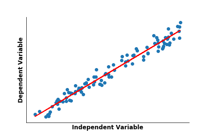 Linear regression is a baseline model which views the dependent variable, Y, that you are trying to predict, as a linear combination of the inputs fed to the model. Linear regression models tune the coefficients for each of these input features to determine their influence on the output.
This is done by minimizing the distance between the training points and the regression model’s line of best fit and is known as Ordinary Least Squares (OLS). OLS has many variants which introduce additional restrictions to reduce over-fitting a model to the noise and anomalies inherent in the training data. The two most common are Lasso and Ridge regression. Another adaptation, logistic regression, allows one to predict labels and categorical variables rather than numeric values.
K-Nearest Neighbors:
While linear regression is mathematically powerful, a more intuitive supervised learning algorithm is K-Nearest Neighbors (KNN). As its name implies, KNN uses the datapoints most similar to the input data in order to output a prediction. The user specifies the number of datapoints to consider. For example, one could specify to K=10, in which case the 10 closest training points to the data of interest would be used to predict the value of interest. This applies naturally to both classification tasks where one wishes to predict a category, such as the genre of a song, and to predicting numeric values, such as home sales. For predicting numeric values, this is often done by taking a weighted average of the nearest points based on their proximity to the input data.
Examples of Unsupervised Learning
Unsupervised learning algorithms are given data which is then transformed into new groupings or representations. These algorithms can highlight structure within the data from an insightful perspective.
Common examples including grouping data and dimensionality reduction. Grouping data is also known as clustering, where an algorithm will partition observations into homogenous groups — group-members have similarities and more in common with other members of their group than individuals from the other clusters formed. [Add intro statement on dimensionality reduction]
Clustering:
For example, let’s say you had a Customer Relationship Management (CRM) database. Clustering customers into distinct groupings could provide valuable insights for developing marketing campaign strategies targeted to the unique needs associated with each of these sub-groups.
An analogous algorithm to KNN for clustering datapoints is the K-Means algorithm. Rather than specifying the number of nearby points, K specifies the number of groups desired to partition the dataset into. From there, clusters of nearby data-points are formed. The process is admittedly a bit more complex than KNN.
The algorithm works by first choosing K random starting points. It then assigns all of the data points to a group based on which of these random starting points it is closest to. After this initial sorting, the centroids of these groups are calculated, and points are then reassigned based on which of these centers they are closest to. (Often this will be the same group, but some points will shift based on the updated centers vs the initial random points.)
This process continues until stabilization when points do not jump groupings and the centroids are solidified. Take a look:
Notice how the cluster centroids, pictured in red, continue to adjust and move. As they do, points that are on the edge of 2 clusters begin to shift where they fall. It should also be noted that this mock dataset naturally clusters into 3 blobs. However, the number of clusters is determined by the user ahead of time. Often this means trying out multiple values for the number of clusters and selecting the result which is most appealing.
Dimensionality Reduction:
The second common type of unsupervised learning algorithms is dimensionality reduction techniques, which compress the data while preserving as much information as possible in this constrained size. These algorithms are often used a preprocessing step within a larger data pipeline, as the compressed data representation often provides practical benefits for training machine learning algorithms.
As mentioned, dimensionality reduction techniques are often an important preprocessing technique before using additional machine learning algorithms. This can be important because while more features will generally improve the accuracy of a supervised learning algorithm, too many can make training the algorithm computationally expensive, or infeasible.
Dimensionality reduction techniques allow you to harness much of the information contained in large datasets with a high number of features, while compressing these details into a manageable size which fits within the resource limitations available. Put simply, it is faster and requires less processing power to train a machine learning model on these compressed representations.
Principal Component Analysis:
One of the most famous examples of dimensionality reduction is Principal Component Analysis (PCA). PCA helps to derive the maximum information from the data using the least number of features. It’s the same idea behind data compression. PCA will reduce the number of dimensions down to a specified number by creating new feature dimensions that account for the most variability within the data. A caveat is that these new features are then difficult to interpret.
In the housing example, a standard regression model would give clear takeaways as to what variables influenced the price of a home.
For example, the model might read house price = n_bedrooms * a + n_bathrooms * b + square_footage * c. Since our features have a clear translation to the real world, the coefficients themselves (a,b, and c) also have clear meanings. If the value of b where 30,000, for example, then the model would imply that a home increases in value by $30,000 for every additional bathroom it has. PCA has tremendous value when large numbers of variables make model training impractical, but the hybrid features it produces have no direct translation back to the context at hand.
In Summary:
Supervised and Unsupervised are two major classifications of machine learning algorithms. Supervised learning algorithms are designed to predict some value or label and require previous examples to do so. Unsupervised algorithms transform data into new representations, such as clustering or dimensionality reduction. While there are a multitude of algorithms that fall into either camp, having a general understanding of how these techniques fall into a larger data strategy is foundational.
To summarize, supervised learning algorithms attempt to predict some value or label given other relevant information. You need previous examples where you know this value or label to train the machine learning algorithm. These prior examples supervise the algorithm.
Unsupervised algorithms do not require this dependent-independent variable split set-up. They do not predict a value or label, but rather reorganize or transform the dataset to unveil underlying structure. The two most common types of unsupervised algorithms are clustering and dimensionality reduction.
About Chisel Analytics:
At Chisel Analytics, our mission is to help companies make progress along their analytics roadmap. Our advisory and staffing services can help your company determine the best applications and strategy for your information, and help you find the temporary or permanent staff you need to move forward. Looking for your next data science role? Join our network of talented data professionals today.
See what others are saying
Let’s stay in touch
You may not be ready for us now, but you’ll want to remember us when you are. Enter your email to stay updated on the latest in analytics and our services.